Developing a Mixed-Signal Simulator

My doctoral research has become very “mixed-signal” in nature. Mixed-signal means there is a lot of interaction between digital and analog signals in a circuit. Even though I have access to state-of-the-art mixed signal simulators, these are expensive luxurious tools and there is no guarantee I will have access to them in the future. So I would like to create a free, open-source one! There are good open-source Spice and HDL (digital) simulator available, so what is needed is integration. This will happen in Python (a scripting programming language).

So how does a mixed-signal problem look like?

Case #1

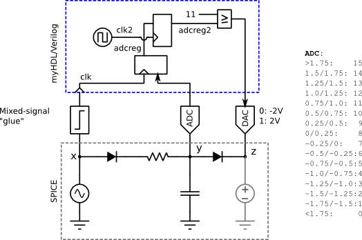
case1_schem

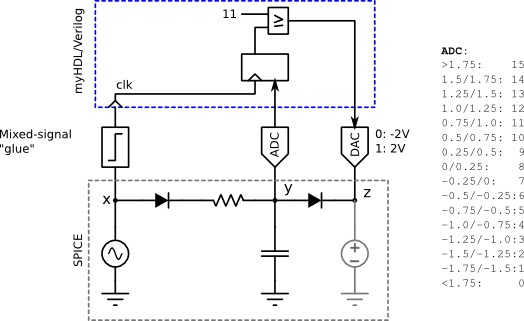
As you can see, there is an analog circuit (bottom), a digital circuit (top) and some “glue” logic that provides a bridge between the analog and digital parts. “Events” determine when each simulation, spice or HDL (digital), is paused, and equivalent values are converted from one domain to another.

In this circuit we have 3 different “glue” elements. The first is a comparator which looks at the analog value in a spice node and waits for it cross a threshold (V(x) > or < 0 Volts). This is the “event”. Then a logic ‘0’ or ‘1’ is set on the digital signal ‘clk’. The second is an ADC (Analog to digital converter) which simply reads the analog voltage at a node and converts is to a digital value. The “event” for this conversion is the rising edge of the ‘clk’ signal clocking the register that will hold the value of the ADC. Finally, a DAC (Digital to analog converter) translates a digital word into an analog voltage. The “event” when this happens is a change in the digital input to the DAC.

Notice the voltage source in gray on the far right. It is “paired” with the DAC to supply the voltage at the DAC to the analog circuit. It’s voltage is changed according the the value of the DAC.

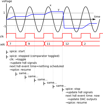
The diagram below describes how a simulation would run:

case1_curves

This is a relatively simple case because the only event is the transition of the comparator, when V(x) goes from negative to positive and vice versa. All updates, to the analog and digital circuits, occur when the spice simulation stops for this condition. Naturally, the clock (clk) is updated, the ADC register is updated because it is clocked by the same ‘clk’ signal, and so is the output of the DAC. No events are expected on the digital side until the comparator triggers again.

The following example illustrates the complexity that can arise when events are expected in the digital side before the spice simulator stops again.

Case #2

Consider this change in the digital circuit:

case2_schem

The register of the ADC is “re-timed” in a second register by a different clock (clk2). Situations like this are not uncommon.

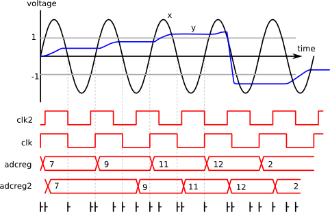
Let’s look at how this would run:

case2_curves

The effect of the change is that there is some small delay and the capacitor is discharged a little later.

The simulation sequence gets complicated from the very beginning. Say we start the HDL simulation first. Then the first event would be the rising edge of ‘clk2′. After that, we start the spice simulator and realize that the rising edge of ‘clk’ happened earlier. Then we need to reset or re-run the HDL simulation from the beginning and stop at the time of the rising edge of ‘clk’ to compute it’s correct state before the rising edge of ‘clk2′ happens.

The penalty of re-simulating a small time interval of HDL might be small, but the provisions to reset the HDL simulation to an earlier state need be available, otherwise the simulation would have to run again from the beginning.

One might infer that the cause of this problem is the fact that there is a clock source in the spice circuit and another in the HDL circuit. One solution to this could be to define all independent “event sources” in just one of the two domains.

Case #3

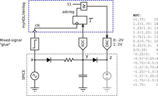
The problem presented in Case #2 can still happen even if “event sources” are only present in the spice side. Consider the small modification to Case #1 where the ADC register has a small delay τ.

case3_schem

The waveforms look like this:

case3_curves

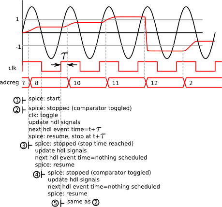
The spice simulation stops on the first rising edge of ‘clk’ (event 2) just as in the previous cases, but now we need to run the HDL simulation until the next event in order to know when the next event will happen (τ seconds later). This way we can resume the spice simulation and instruct it to stop at the time of the next event (event 3). Previously, we instructed the spice simulator to stop only when the comparator triggered. Now we are instructing it to stop at a specific time.

The problem here is that the comparator could toggle before the specified stop time. This would require an update of HDL signal, and potentially, the previously scheduled event might not even happen (or happen at a different time). So we need to discard the scheduled events, and run the HDL simulation again.

This has been a first approach to understanding the complexities in synchronizing analog and digital simulators for implementing a mixed-signal simulators. Comments are appreciated as well as any other contribution towards this project.

Impact of the Magnetic Levitator

The video below shows no magic. It’s a simple and beautiful example of engineering.


Making a piece of metal float in the air is the combination of the understanding and clever manipulation of basic forces of nature to accurately produce desired results. This is probably a general description of what engineering is all about. This particular example has always amazed me though, because it seems to defy nature, it combines several engineering disciplines, and at the same time, is relatively simple. Show this to someone thinking of becoming an engineer!

So let me explain it. The big picture first. The sub-discipline of electrical engineering that deals with “keeping or putting things where you want them” is called Control Systems. The simplest example is the temperature control of your heating/cooling system at home. You set your desired temperature and the thermostat looks a the current temperature. The difference is the “error”. It is used to decide what to do. If it is positive (the desired temperature is higher than the actual), it turns on the heating. If it is negative, the it turns it off. This keeps the temperature where you want it.

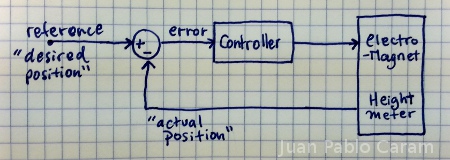
For the magnetic levitator the situation is similar. The setting is the desired position of the suspended mass. The controller looks at the current position to compute the position error. If the mass is too low, it increases the force on the electromagnet above, otherwise, it decreases it.

The figure below shows a diagram of the system:

controls

Boxes and arrows are the alphabet of electrical (and other) engineers. So what you see above is an explanation of the magnetic levitator in electrical engineering language. The arrows are signals. Signals are some quantity, magnitude, or intensity. The boxes are operations, which receive signals, do something with them, and output new ones.

“Desired position” and “actual position” are signals of the same kind, height of the levitated object”m so we can carry out a subtraction operation, represented by the circle with “+” and “-” symbols. The “error” is the result of the operation. It is the input to “Controller”, whose task is to set the intensity of the electromagnet in such a way that the object levitates, or that the “error” becomes zero (or constant right?)

The operation done by the “Controller” to establish the intensity of the electromagnet based on the error is quite simple, but perhaps too advanced to be relevant to this writing. The point is that the operation is just well known math at the calculus level.

So the question that probably remains is what are the signals and operations made of? My answer is that it doesn’t really matter much (up to certain point, to the control systems engineer). He can design and test this on the computer. But if we want to build it we need to explore some other areas in electrical engineering. Keep in mind that certain parts of the levitator could be implemented as a program on a computer, but let’s assume we want to completely build it with analog circuits. The analog circuit designed (a specialized electrical engineer) uses operational amplifiers to do math. Operational amplifiers are one of the oldest and most used circuits ever. So the “operation” boxes are made with one or more operational amplifiers. The signals are typically voltages or currents (stuff that moves on wires.) Conveniently, the arrow and boxes in the drawings resemble the real thing in circuits, this is, wires and chips!

What you see in the video too me and a friend just a couple of hours to build (after knowing what parts we would need and making sure we had them ready.) It required almost no math at all. It is not that complicated. After this, you can go after much harder tasks… google “Inverted pendulum” and watch some videos.

Control Systems is what is behind the autopilot in a passenger jet, what keeps a “segway” standing despite having only two wheels, and what keeps many things running smoothly and safely without you ever noticing. I hope this writing serves as some inspiration!

Free and Open Source Software for Electrical Engineering

Throughout the years I’ve used hundreds of software tools to do my job and research. Many of these are extremely expensive and I’ve only had access to them through school or employers. Some of these are Matlab, the Cadence tools, Agilent ADS and Ansys HFSS. Becoming proficient in their use is a major investment, and there is no guarantee that you will have access to them in the future.

Learning open source tools is a much better personal investment. This does not mean that you are better off leaning these instead of Cadence if you need it for your job, but if you have spare time to get good at your tools, some of those that I describe here might yield a higher return in the future.

Scientific Computing

Python, Scipy, Numpy and MatplotLib vs. Matlab: Python has rapidly become the most popular scripting language in the world. There is such a large community of users, that there is probably more libraries and documentation than what you’ll even need. Scipy, Numpy and Matplotlib are libraries that simplify numerical computation and creating plots.

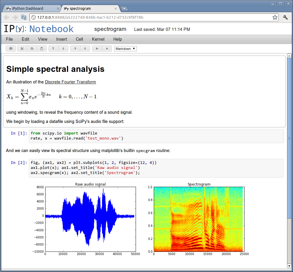
iPython notebook is a spectacular tool that integrates several tools built around Python that provide the most powerful scientific computation environment that I’ve ever used. Click on the image below to go to the iPython Notebook website:

iPython Notebook

The easiest way to install all the tools together is by following the instructions at scipy.org.

Circuit Simulation

LTSpice: Not open source but free. Features schematic capture, SPICE simulator and  waveform viewer. This is a simulator you can trust. Some of my school mates at Georgia Tech use it for IC design!

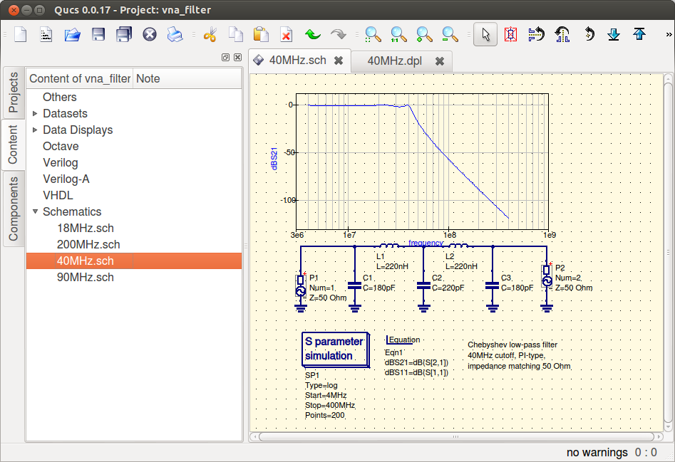
QUCS: This is probably the most ambitious project in this category. It integrates schematic capture, a rich results viewer, and simulators for transient, AC, S-Parameter, Verilog, and others all together! Its interface imitates some of the feature of Agilent ADS, which allows for very good integration.

QUCS

CircuitLab: An online circuit simulator (Schematic capture, transient and AC simulation, and plots). It’s closed and limited in features, but very well designed. It provides an excellent interface and robust features for circuits of low complexity. In this sense it it an excellent learning tool. As it is the trend on online applications, it allows sharing your designs.NGSpice:

HDL Simulation

IVerilog: Open-source verilog simulator based on IEEE Std 1364-2005. Binaries available for Linux, Windows and MacOS. Fast and maintained actively. Compiles files for simulation, RTL synthesis and some target FPGAs.

GTKWave: Mature waveform viewer. Biaries for all platforms. Supports analog and digital signals together.

Impulse: VCD waveform viewer plug-in for Eclipse. Has more features than GTKWave, and its integration with Eclipse speeds up the design process.

PCB Design

KiCad: Combines schematic capture, layout editor (forward and back-annotation between the two), library editor and Gerber viewer. This is a professional-grade EDA application, actively developed, and features advanced capabilities like auto-routing, design rule check (DRC) and scripting (in Python.)

KiCAD

PCB: The other big player in the open-source PCB world. PCB is part of the GEDA project. More to come…

Authoring

Inkscape: A significant amount of engineering knowledge is shared through drawings and diagrams. Inkscape is a vector-graphics drawing program that has all the features you will ever need. Wether you want to draw a block diagram, circuit schematics, or annotate plots generated with other tools (like Matplotlib above), it will be more that suitable for the job and you will be delighted by the quality of the final result. It features a flexible plugin engine and tons of plugins are available, such as LaTeX input, which will allow you to create vector graphic equations and embed them in your drawing!

Lyx: LaTeX made easy! Lyx is a LaTeX editor that makes most LaTeX features available through its graphical interface and hides LaTeX code in your documents by providing a preview render instead. This allows you to see your document’s outline, equations and images. It is not a WYSIWYG editor, but more of a convenience interface to compose your documents faster and avoid writing LaTeX most of the time, but still providing access to the code for faster access when you dominate the language. If you want LaTeX quality output but don’t have the time to learn the language right now, this is the tool you need.

Others: writelatex.com

Do you LaTeX?

Writing pretty documents is not an easy task if you use a word processor. You will invest a great part of your time focusing on the visual aspects of your document rather than on the content. This is not trivial for engineering, science and math, students and professionals.

LaTeX will get you there.

A document compiled using LaTeX.

LaTex is a document compiler. This means you write plain-text code and LaTeX will generate your document (PDF and other formats) from it. This allows you to focus on content, while LaTeX takes care of the rest.

Learning the LaTeX language and setting up LaTeX tools can be a scary task and too big of a project when your paper was due yesterday. After you’ve invested the time to learn though, the benefits are quite rewarding.

To minimize the cost of the initial investment, I would like to share 2 tools that can get you started very quickly. These are Lyx and writelatex.com.

Lyx is a desktop program that runs on Windows, Mac OS and Linux, and allows you to access all of LaTeX’s functions through a menu-driven interface, while also displaying your document like a standard text processor. The advantage of this, is that you are not looking at LaTeX code, but just the contents of your document. The installation program will take care of downloading all the tools you might need, and will provide support for generating almost any imaginable format, including PDF, as well as support for every image format. Another nice benefit of Lyx is that it support copying and pasting from other documents, so there is no need to manually transform your images, for example, into standalone files in appropriate formats.

WriteLaTeX, on the other hand, is a web-based LaTeX editor. It requires you to write LaTeX code, but it shows you the resulting document side-by-side with your code so you don’t have to manually compile to see how your document will end up looking. This tool has all the nice benefits of web applications, like not having to install anything on you computer, and being able to share and collaborate on documents. WriteLaTeX makes it easy to upload images and data to your document, not just from your PC but from DropBox and Google Drive, thus making it a fully cloud-based app!

Both tools are free, so you can start using them right now!

uControllers have evolved!

It’s been a while since I worked with microcontrollers and I wanted see what’s around today. I was used to 8-bit PICs, because they where cheap, as well as the programmers (you could make your own in less than an hour), and because of the great range of available development environments.

But things have changed! 32-bit micro’s are so cheap now, and most manufacturers have realized that they must provide their development tools for free. So I purchased a $99 32-bit PSoC ARM development board from Cypress.

CY8CKIT-050 PSoC® 5 Development Kit (First test)

But the PSoC (Programmable System on Chip) is not just a powerful microcontroller, it’s also a CPLD and a programmable analog circuit containing op-amps, mixers, DACs, ADCs, filters, etc. In addition to that, their IDE (Integrated Development Environment) is excellent, unlimited and free. No need to guess how to setup anything, the graphical environment is self explicative and context-relevant documentation is a button-click away.

Thank you Cypress!